Should You Do A Search Fund?.
A decision framework for someone considering the search fund path: intellectually thorough, complete, and detailed enough to pressure-test the choice before committing years to it.
Should You Do A Search Fund?
Search funds used to be a genuine edge case in the alternatives universe. They are more crowded now. Entry multiples have drifted from 5× to 7× EBITDA over the past decade, which compresses every return scenario. Running a small business is genuinely hard in ways that no model captures cleanly. And that is assuming you find a deal at all – 37% of concluded searches never close one.
This post works the problem from the bottom up: a deterministic LBO as the kernel, a probability-weighted scenario tree wrapped around it, and 500,000 Monte Carlo trials calibrated to Stanford's published base-rate data – followed by a decision framework built from the output. The exhibits are interactive and detailed enough for a technically-minded reader to pressure-test every assumption.
The median search-fund outcome does not beat a strong W-2 counterfactual. The decision only gets interesting when you have a concrete edge that plausibly moves you toward the right tail – and you have to be honest about whether you actually have that edge before you commit two years of your life to finding out.
Structure, base rates, fit, and failure modes. Before the analysis has anything useful to say, the search-fund instrument has to be defined.
TL;DR
- A search fund raises investor capital to buy and operate one small business as a first-time CEO.
- Expect roughly 3–6 months fundraising, 18–24 months searching, then 5–10 years operating before exit.
- Key risks are failing to acquire, overpaying, operational underperformance, leverage stress, and delayed or weak exits.
- Best for resilient operators seeking concentrated upside; poor for people needing predictable income or low uncertainty.
A compact 3-question rubric
Before you go deeper into the asset-class history or model mechanics, pressure-test your fit across three dimensions: duration risk, opportunity-cost risk, and operator-market fit.
1) Can you tolerate 2 years with no close?
- Green: You can absorb ~24 months of search uncertainty (and possible no-deal outcomes) without destabilizing your finances, relationships, or conviction.
- Yellow: You can handle the timeline only with constraints (tight cash runway, geography limits, or reduced flexibility on target quality).
- Red: A prolonged search or failed close would create unacceptable personal or financial stress.
2) Is your outside option below your personal break-even threshold?
- Green: Your realistic W-2 alternative is clearly below the expected utility you require to justify search-fund risk.
- Yellow: Your outside option is near your break-even line; small misses on timing or outcomes erase the edge.
- Red: Your outside option already dominates once you adjust for risk, time-to-liquidity, and variance.
3) Do you have operator-market fit for small-business leadership?
- Green: You have credible fit for owner-operator work: sales motion, hiring judgment, cash discipline, and stamina in unglamorous execution.
- Yellow: You have partial fit, but key capabilities (deal sourcing, frontline leadership, or turnaround execution) are still developing.
- Red: Your strengths are primarily advisory/analytical, and day-to-day SMB operating leadership is not a natural match.
If you want to quantify each axis before proceeding, jump to Exhibit 1 (search funnel and no-close risk), the decision rule section (outside-option break-even), and Exhibit 4 (operator execution sensitivity).
The asset class
At base, a search fund is an investor-backed path where a first-time operator raises a search pool, acquires one business, and then runs it as CEO. The attraction is concentrated equity upside; this section adds the historical and base-rate context from Stanford.
The best data set on the asset class is Stanford GSB's biennial Search Fund Study. The 2024 edition tracks 681 first-time funds formed in the U.S. and Canada since 1984.
The structure
A search fund has two stages — or four, if you zoom out to the full lifecycle Stanford uses in the study:
| Stage | Typical duration | What's happening |
|---|---|---|
| 1. Raise initial capital | 3–6 months | Searcher raises ~$500k from 15–25 investors |
| 2. Search & acquisition | ~18–24 months | Hunt target; negotiate; close |
| 3. Operation | 5–10 years | Searcher runs the company as CEO |
| 4. Exit | — | Sale, recap, or other liquidity event |
Stage 1 — Raise initial capital. An individual or two-person partnership raises the search pool, typically $400k–$700k from 15–25 investors. The capital funds salary, travel, diligence, and legal work while the searcher builds the acquisition funnel.
Stage 2 — Search and acquisition. The searcher sources targets, submits indications of interest, signs LOIs, runs diligence, negotiates financing, and closes one company if the process works. At close, the original investors usually have a pro-rata right, not an obligation, to fund the acquisition equity.
Stage 3 — Operation. The searcher becomes CEO, runs the company for 5–10 years, and tries to turn a good small business into a more durable and valuable one. The searcher’s equity upside usually lands in the 20–30% range after full vesting.
Stage 4 — Exit. The company is sold, recapitalized, or otherwise converted into liquidity. This is where the searcher’s equity value is realized, and where most of the personal financial variance lives.
The searcher's equity vests on three tranches: 1. Time vesting over four to five years 2. Acquisition vesting earned at close 3. Performance vesting tied to IRR hurdles at exit
Total searcher equity at exit typically runs 20–30% after full vesting.
What the CEO actually gets paid
Searcher equity is the prize, but there's a steady cash component too. Stanford's 2024 study reports median CEO cash compensation (base + bonus) by tenure, across 149 reporting companies:
| Years since acquisition | Median base | Median bonus | Median total |
|---|---|---|---|
| ≤ 1 year | $190k | $25k | $200k |
| 1–2 years | $210k | $55k | $262k |
| 2–3 years | $215k | $50k | $265k |
| 3–4 years | $225k | $67k | $292k |
| 4–5 years | $205k | $29k | $226k |
| 5+ years | $229k | $45k | $260k |
Cash comp is deliberately modest. The point of a search fund is not to get rich on salary; it's to earn a meaningful equity stake in a company you control.
Variants
The traditional structure is one of three variants worth distinguishing:
- Traditional search fund. Investor-funded search, investor-led acquisition equity, structured governance, 20–30% searcher equity at exit. The default in the Stanford data set.
- Self-funded search. No outside search capital and no salary during the hunt. The acquisition is financed with an SBA 7(a) loan, a seller note, and personal equity. SBA 7(a) lends up to $5M for a business acquisition at roughly 10% equity down. The searcher keeps full equity and answers to no board; the trade is the unpaid search and a personal guarantee on the SBA debt.
- Independent sponsor. Source the deal first, raise the equity for it from a network of capital partners after. Closer to a one-deal private-equity spinout than a search fund proper.
All three converge on a similar target profile but diverge sharply in execution. Pick one before you start sourcing: your diligence process, lender conversations, and seller narrative all change with the structure.
The target profile
The canonical search-fund target:
- Revenue $5M–$30M
- EBITDA $1.5M–$5M
- Recurring or highly repeat revenue
- Owner retiring, no clear successor
- Boring, stable, unglamorous industry
- Fragmented market (roll-up optionality, or protection from new entrants)
The thesis is simple: these companies are too small for traditional PE, too large for individual entrepreneurs, and their owners are aging out. A new operator with capital and energy can meaningfully improve them.
Stanford's 2024 data reports median statistics for all 328 acquisitions tracked through 2023 and the 2022–2023 cohort specifically:
| Median | All acquisitions | 2022–2023 |
|---|---|---|
| Length of search | 19 months | 20 months |
| Purchase price | $12.8M | $14.4M |
| Revenue at purchase | $7.3M | $6.7M |
| EBITDA at purchase | $1.9M | $2.2M |
| EBITDA margin | 22.8% | 26.9% |
| EBITDA growth rate | 11.4% | 25.0% |
| Purchase multiple | 6.4× EBITDA | 7.0× EBITDA |
| Employees | 40 | 34 |
Two things jump out. First, multiples have compressed the margin for error — the median has drifted from ~5× a decade ago to 7× in the most recent cohort. Second, the 2022–2023 cohort is skewing toward higher-margin, faster-growing, smaller-headcount businesses — a reasonable response to richer entry prices.
Historical returns
Stanford GSB's biennial Search Fund Study is the canonical data set. The most recent edition shows:
- Aggregate IRR: mid-to-high 30s
- Aggregate MOIC: ~5–6×
- Success rate: roughly 60% of funds that close an acquisition return capital; about 30% generate outsized returns; about 10% are total losses
Those are cohort-level numbers. Individual outcomes are strongly bimodal: a few home runs, a solid middle mass, and a meaningful tail of zeros.
The outcome tree
Stanford's outcomes tree makes the bimodality explicit. Concluded search funds (100%) split first into no acquisition (37%) and acquisition (63%).
Of the 63% that made an acquisition:
| Outcome | Share of acquisitions |
|---|---|
| Gain | 69% |
| Loss | 31% |
Inside the gain branch:
| ROI bucket | Share of gains | % exited | Hold (exited) |
|---|---|---|---|
| 1–2× | 27% | 23% | 5.8 years |
| 2–5× | 36% | 66% | 4.9 years |
| 5–10× | 25% | 84% | 5.2 years |
| >10× | 11% | 61% | 10.3 years |
The ≥5× outcomes do most of the work. Losses exit faster than wins. Roughly half of concluded funds don't meaningfully return capital. The ~25% of funds in the ≥5× range are carrying the asset class.
You should do a search fund only if your plan plausibly reaches the ≥5× branch, because that tail is what pays for the large no-deal and loss branches.
Why it works (when it does)
- Supply-demand on small companies. Most traditional buyers skip deals under $10M of EBITDA because transaction costs don't justify sub-$50M acquisitions. Sellers in this range are frequently choosing between a searcher, a strategic, and no sale at all.
- Asymmetric upside for the searcher. Two-year salary floor with equity-like upside on the back end.
- Strong governance. Investor board seats, acquisition rights, and structured oversight reduce the "first-time CEO runs the company into the ground" risk.
- Small size is an advantage. At $3M EBITDA, small operational improvements have disproportionate impact on multiple-adjusted returns.
Why it fails (when it does)
Most failures are execution failures under pressure, not spreadsheet failures at signing. The same patterns recur across outcomes: late-cycle capitulation, concentration risk disguised as stability, hidden owner dependency, and leverage fragility under even modest drawdowns.
- Bad acquisition. The #1 failure mode: capitulation. After 18 months of searching with no deal, the psychological pressure to close leads searchers to buy inferior companies they initially rejected.
- Customer concentration. A "recurring revenue" business where 60%+ of revenue is concentrated in the top three customers is not recurring in the sense that matters.
- Hidden owner dependency. The retiring owner was the relationship, the culture, and the operations. When they leave, the business unravels over 18 months.
- Debt service in a downturn. Leveraged capital structures are fragile. A 20% revenue decline that an unlevered operator absorbs is terminal for a 70% leveraged one.
- The searcher is the wrong operator for the business. Pattern-matching between searcher profile and target profile is underrated.
Diligence, financing, and the first 90 days
Once an LOI is signed (60–90 day exclusivity, non-binding except on shopping), the diligence budget on a sub-$5M deal runs $30k–$50k: quality of earnings ($15k–$30k) and legal ($15k–$20k).
For SBA-financed deals, run the loan in parallel with diligence — both take 8–12 weeks regardless of sequencing. Roughly two dozen banks nationally specialize in SBA acquisition lending; using one of them compresses the timeline by about two months versus a generalist.
The single most repeated piece of post-close advice from operators: change nothing in the first 90 days that you do not absolutely have to. Employees are watching closely, and early changes signal who you are before you've earned the credibility to make them stick.
Who it's for
The structure rewards a very specific profile: operationally-minded, high agency, comfortable with ambiguity, willing to live unglamorously for two-plus years during the search, and able to make a ten-year commitment to a small company in a boring industry. If any of those doesn't describe you, the better path is probably traditional operating roles or direct-to-deal investing.
Treat profile fit as a hard filter before underwriting returns. If you fail the profile test, skip the analysis even if the upside math is attractive on paper.
From here on, simulation scope is the traditional search-fund model. The taxonomy, assumption map, and layer stack define that baseline before the distributions appear.
Which model are we simulating?
The simulation in this post is explicitly the traditional search-fund model. Traditional, self-funded, and independent sponsor searches differ on who provides search capital, how operator equity vests, and what governance constraints apply. The exhibit below locks that scope before we interpret any outputs.
The three models of entrepreneurial acquisition
The asset class is not monolithic. Search capital, salary, equity, and governance differ materially across these three paths. All downstream simulation results in this post assume the traditional model column.
| Dimension | Traditional | Self-funded | Sponsored (PE-backed) |
|---|---|---|---|
| Search-capital source | 10–15 outside investors | Searcher's personal capital | Single PE firm (EIR model) |
| Typical search capital | ~$400K–$550K | $0 raised externally | Firm covers full cost |
| Search-stage salary | ~$94k–$139k (region-dep.) | None — personal savings | $150k–$200k |
| Typical search duration | ~19–23 months | Variable; one anchor at 6 mo | Variable; one anchor at 11 mo |
| Acquisition capital | Same investor base + new LPs | Bank debt + small equity slice | PE sponsor majority |
| Step-up on conversion | ~150% of search investment | n/a | n/a |
| Searcher equity | 20–30% common (solo 20–25, partner 25–30) | Majority — direct ownership | 15–20% incl. performance |
| Vesting structure | 3 equal tranches: time / acq / IRR-perf | Not vested — owned at close | 3 tranches incl. performance |
| Performance hurdle (T3) | 20% IRR (0% vest) → 35% IRR (100%) | n/a | Set by sponsor |
| Governance | Distributed; investor right of first refusal | Founder retains control | Sponsor majority + 3 of 5 board seats |
| Closure rate | ~63% of concluded acquire (US) | Higher — owner controls timing | Typically completes |
| Anchor case | Brown Robin / OnRamp Access | Sanabria / Impress Northwestern | Callahan / YLighting (Alpine) |
| Active case | Traditional search fund | Not used | Not used |
Scope. Everything in this post sits in the Traditional column above. Re-running the simulator under self-funded or sponsored assumptions would shift the searcher-take histogram materially.
| Assumption | Baseline | Source/Anchor | Why it matters |
|---|---|---|---|
| Entry multiple | 7.0× EV / EBITDA | Layer 1 intro; static workbook snapshot; search-fund-lbo/01-sources-and-uses |
Sets purchase price and equity check; most direct MOIC/IRR lever. |
| Leverage | 40% senior debt + seller note | Layer 1 intro; search-fund-lbo/01-sources-and-uses; search-fund-lbo/03-debt-schedule |
Controls equity at close, debt service burden, and downside fragility. |
| Revenue growth path | Deterministic central path (vol = 0) | Layer 1 intro; search-fund-lbo/02-operating-model; search-fund-lbo/06-driver-appendix |
Primary driver of EBITDA expansion and terminal value under fixed exit multiple. |
| Margin path | Deterministic central path (vol = 0) | Layer 1 intro; search-fund-lbo/02-operating-model; search-fund-lbo/06-driver-appendix |
Converts top-line into EBITDA; key interaction with debt paydown capacity. |
| Exit multiple | 7.0× EV / EBITDA (no expansion) | Layer 1 intro; search-fund-lbo/04-returns-waterfall; search-fund-lbo/05-sensitivity-tables |
Defines terminal enterprise value; determines how much growth translates into cash-out. |
| Hold period | 5.5 years | Layer 1 intro; search-fund-lbo/04-returns-waterfall |
Affects IRR denominator, debt amortization runway, and vesting realization timing. |
| Salary counterfactual | $3.0M cumulative W-2 baseline | Static decision benchmark used in the lede, Exhibit 2, Exhibit 4b, and the counterfactual readout panel. | Decision threshold: converts outcomes into opportunity-cost-adjusted personal economics. |
Why a single-point model lies
Search-fund outcomes are branchy rather than linear: no-acquisition risk, loss branches, and a right tail that carries aggregate returns. A single-path LBO summary mis-specifies the decision. The analysis has to be distribution-first.
The deterministic model is the right place to start. It gives you the kernel — the mechanics of the deal, the capital structure, the waterfall, the sensitivity table. But a kernel is not a conclusion. Layer 1 by itself simply cannot carry that weight. So we add the next two layers.
Simulation assumption map
A compact read of the core inputs used across Layer 2 and Layer 3. Each row names the default, why the base case is set there, and the directional effect on searcher IRR if the input moves.
| Assumption | Default used | Why this base case | IRR if higher | IRR if lower |
|---|---|---|---|---|
| Entry multiple | 7.0× EV / EBITDA | Anchors to the Layer 1 kernel so all realism penalties are measured off a constant underwriting frame. | ▼ | ▲ |
| Exit multiple | 7.0× EV / EBITDA | No expansion/contraction base case isolates operating execution from valuation drift. | ▲ | ▼ |
| Leverage % at close | 40% senior debt (+ seller note) | Matches the deterministic cap structure used in Layer 1 and keeps downside fragility explicit. | ▲Usually, until distress risk dominates | ▼Usually, with less tail risk |
| Search duration | 2 years pre-close salary drag | Simple representation of the pre-acquisition burn before outcome branches are realized. | ▼ | ▲ |
| Outside-option salary path | $3.0M cumulative W-2 counterfactual | Decision benchmark from the post framing; converts outcomes into opportunity-cost-adjusted personal returns. | ▼Relative attractiveness | ▲Relative attractiveness |
| Vesting / equity share | Three-tranche searcher vesting grid | Reflects standard search economics; payout only scales when value creation and time thresholds are met. | ▲ | ▼ |
The deterministic LBO is the kernel, not the answer. The next layer adds base-rate branches, search friction, and the path from a single case to a distribution.
The three-layer stack
The simulator is not one approach — it is three, stacked. Each layer is the previous layer with one piece of honesty added back.
The engine every searcher builds in Excel. One purchase price, one growth path, one exit multiple, one waterfall, one searcher take. On the canonical Stanford-median deal it returns an investor MOIC of 2.68× and an IRR of 19.6% over a 5.5-year hold; the searcher walks away with $4.56M pre-tax. Useful as a kernel. Dishonest as a summary, because it presents a single trajectory through a stochastic world as if it were the answer.
Wrap Layer 1 in Stanford's published outcome buckets — no acquisition, total loss, partial loss, 1–2×, 2–5×, 5–10×, >10× — weight each branch by its observed frequency, and sum to an expected value. The deal-level 2.68× MOIC collapses to roughly 2.33× and 16.6% IRR once the no-acquisition and loss branches are paid for. This is what a competent PE memo does. It is what almost no first-time searcher spreadsheet does.
Replace the seven discrete buckets with continuous distributions on the twelve operating drivers, calibrated so the emergent bucket frequencies match Stanford 2024 in aggregate. Run 500,000 trials. The output is not a number — it is a histogram. Where the mass sits, where the tail sits, and how the searcher's pre-tax NPV reads against a $3M W-2 counterfactual is the only thing in the analysis that actually answers the question.
Layer 1 — the deterministic kernel
The six exhibits below are the deterministic-mean trial of the same Rust engine that runs the 500,000 trials later in the post — i.e. the simulator with vol_multiplier = 0 and every driver pinned at its central value. A $13.51M purchase price on $1.93M of starting EBITDA, 40% senior debt, a seller note, three searcher vesting tranches, exit at year 5.5 on the same multiple. Sources & uses, the operating model, the debt schedule, the returns waterfall, a sensitivity table, and the full driver appendix. Read these as the kernel; the distribution shown later is built by sampling around exactly these inputs.
Workbook
Static workbook snapshot behind the six deterministic exhibits below.
6 sheets · sources and uses · operating model · debt schedule · returns waterfall · sensitivity tables · driver appendix
| Driver / line | Yr 0 (close) | Yr 1 | Yr 2 | Yr 3 | Yr 4 | Yr 5 | Yr 6 (exit) | Source |
|---|---|---|---|---|---|---|---|---|
| Drivers | ||||||||
| Customer count (BoP) | 1,000.0 | 1,040.0 | 1,081.6 | 1,124.9 | 1,169.9 | 1,216.7 | 1,265.3 | Y0 driver |
| Annual churn | 9.0% | 9.0% | 9.0% | 9.0% | 9.0% | 9.0% | 9.0% | Driver |
| New customer adds % | 13.0% | 13.0% | 13.0% | 13.0% | 13.0% | 13.0% | 13.0% | Driver |
| ARPU ($) | 7,000.0 | 7,426.1 | 7,878.2 | 8,357.8 | 8,866.6 | 9,406.3 | 9,978.9 | Y0 driver |
| Price growth % | 3.5% | 3.5% | 3.5% | 3.5% | 3.5% | 3.5% | 3.5% | Driver |
| Volume-per-customer growth % | 2.5% | 2.5% | 2.5% | 2.5% | 2.5% | 2.5% | 2.5% | Driver |
| Revenue build | ||||||||
| Revenue | 7,000.0 | 7,723.2 | 8,521.1 | 9,401.4 | 10,372.6 | 11,444.2 | 12,626.5 | customers × ARPU |
| Cost stack (negative convention) | ||||||||
| Variable cost (40.0% of revenue) | (2,800.0) | (3,089.3) | (3,408.4) | (3,760.5) | (4,149.0) | (4,577.7) | (5,050.6) | Driver · 40.0% |
| Wages | (1,870.0) | (2,083.4) | (2,321.1) | (2,585.9) | (2,880.9) | (3,209.6) | (3,575.8) | FTE × wage / FTE |
| ↳ Headcount (FTE) | 34.0 | 36.4 | 39.0 | 41.8 | 44.8 | 48.0 | 51.4 | Scales rev0.7 |
| ↳ Wage per FTE ($) | 55,000 | 57,200 | 59,488 | 61,868 | 64,342 | 66,916 | 69,593 | Driver · 4.0% growth |
| Fixed overhead | (400.0) | (412.0) | (424.4) | (437.1) | (450.2) | (463.7) | (477.6) | Driver · 3.0% growth |
| EBITDA | 1,930.0 | 2,138.5 | 2,367.2 | 2,617.9 | 2,892.5 | 3,193.2 | 3,522.5 | Revenue − costs |
| EBITDA margin | 27.6% | 27.7% | 27.8% | 27.8% | 27.9% | 27.9% | 27.9% | Emergent output |
| Capex & working capital | ||||||||
| Maintenance capex (2.5% of revenue) | (175.0) | (193.1) | (213.0) | (235.0) | (259.3) | (286.1) | (315.7) | Driver · 2.5% |
| Growth capex (8.0% of ΔRevenue) | (560.0) | (57.9) | (63.8) | (70.4) | (77.7) | (85.7) | (94.6) | Driver · 8.0% |
| Working-capital change (10% of ΔRevenue) | (700.0) | (72.3) | (79.8) | (88.0) | (97.1) | (107.2) | (118.2) | Driver · 10.0% |
| FCF (pre-tax) | 495.0 | 1,815.3 | 2,010.6 | 2,224.4 | 2,458.3 | 2,714.2 | 2,994.0 | EBITDA − capex − ΔWC |
Full debt schedule Collapsed by default · open for row-level audit
| Line | Yr 0 (close) | Yr 1 | Yr 2 | Yr 3 | Yr 4 | Yr 5 | Yr 6 (exit) | Source |
|---|---|---|---|---|---|---|---|---|
| Senior debt · 8.5% rate · 7-yr linear amort | ||||||||
| Beginning balance | 5,404.0 | 5,404.0 | 4,408.5 | 3,270.2 | 1,973.8 | 502.3 | – | Y0 from Ex. 01 |
| Interest expense @ 8.5% | – | (459.3) | (374.7) | (278.0) | (167.8) | (42.7) | – | BoP × rate |
| Mandatory amort | – | (772.0) | (772.0) | (772.0) | (772.0) | (502.3) | – | $5,404 / 7 |
| Cash sweep (50% of excess FCF) | – | (223.5) | (366.3) | (524.5) | (699.4) | (1,027.7) | – | Excess after int + mand |
| Ending balance | 5,404.0 | 4,408.5 | 3,270.2 | 1,973.8 | 502.3 | – | – | BoP − mand − sweep |
| Seller note · 6.0% rate · 7-yr linear amort | ||||||||
| Beginning balance | 675.5 | 675.5 | 579.0 | 482.5 | 386.0 | 289.5 | 193.0 | Y0 from Ex. 01 |
| Interest expense @ 6.0% | – | (40.5) | (34.7) | (29.0) | (23.2) | (17.4) | (11.6) | BoP × rate |
| Mandatory amort | – | (96.5) | (96.5) | (96.5) | (96.5) | (96.5) | (96.5) | $675.5 / 7 |
| Ending balance | 675.5 | 579.0 | 482.5 | 386.0 | 289.5 | 193.0 | 96.5 | BoP − mand |
| Cash flow check | ||||||||
| FCF (pre-tax) from Ex. 02 | 495.0 | 1,815.3 | 2,010.6 | 2,224.4 | 2,458.3 | 2,714.2 | 2,994.0 | FCF available |
| Total cash debt service | – | (1,591.8) | (1,644.3) | (1,699.9) | (1,758.9) | (1,686.6) | (108.1) | Sum of int + amort + sweep |
Source waterfall table Open for line-by-line audit
| Line | % of equity | Amount ($000) | Source / note |
|---|---|---|---|
| Exit waterfall | |||
| Exit EBITDA (Yr 6) | – | 3,522.5 | From Ex. 02 |
| × Exit multiple | – | 6.5× | Driver · Stanford anchor |
| Enterprise value at exit | – | 22,896.3 | EBITDA × multiple |
| Less: senior debt outstanding | – | 0.0 | From Ex. 03 · paid off Yr 5 |
| Less: seller note outstanding | – | (96.5) | From Ex. 03 Yr 6 EoP |
| Equity value at exit | – | 22,799.8 | EV − debt |
| Searcher vesting waterfall | |||
| Acquisition vest (sweat at close) | 5.0% | 1,140.0 | Tier 1 · vests at close |
| Time vest (10% over 5 yrs) | 10.0% | 2,280.0 | Tier 2 · 5.5y ≥ 5y ⇒ full vest |
| Performance vest (step on investor IRR) | – | – | Tier 3 · three hurdles |
| Hurdle 1 · IRR ≥ 20% ⇒ +5% | 5.0% | 1,140.0 | Cleared · pre-vest IRR 21.0% |
| Hurdle 2 · IRR ≥ 35% ⇒ +5% | not cleared | – | 21.0% < 35% |
| Hurdle 3 · IRR ≥ 50% ⇒ +5% | not cleared | – | 21.0% < 50% |
| Searcher total vested | 20.0% | 4,560.0 | Sum of tiers |
| Returns split | |||
| Searcher take | 20.0% | 4,560.0 | Equity × vested % |
| Investor take | 80.0% | 18,239.8 | Equity × (1 − vested %) |
| Investor returns | |||
| Investor cash invested | – | 6,809.0 | From Ex. 01 · MOIC denom |
| Investor MOIC | – | 2.68× | Take ÷ cash |
| Investor IRR (5.5-yr hold) | – | 19.6% | MOIC1/n − 1 |
| Searcher MOIC (on $0 cash) | – | infinite (sweat basis) | No cash invested |
Investor IRR · entry multiple × exit multiple
| Entry ↓ / Exit → | 5.5× | 6.0× | 6.5× | 7.0× | 7.5× |
|---|---|---|---|---|---|
| 6.0× | 19.5% | 21.4% | 23.2% | 24.8% | 26.4% |
| 6.5× | 19.0% | 19.6% | 21.3% | 23.0% | 24.5% |
| 7.0× | 17.3% | 19.2% | 19.6% | 21.3% | 22.8% |
| 7.5× | 15.8% | 17.6% | 19.4% | 19.7% | 21.2% |
| 8.0× | 14.4% | 16.2% | 17.9% | 19.5% | 19.7% |
Investor IRR · price growth × exit multiple
| Growth ↓ / Exit → | 5.5× | 6.0× | 6.5× | 7.0× | 7.5× |
|---|---|---|---|---|---|
| 1.5% | 13.7% | 15.5% | 17.2% | 18.8% | 19.0% |
| 2.5% | 15.5% | 17.4% | 19.1% | 19.4% | 20.9% |
| 3.5% | 17.3% | 19.2% | 19.6% | 21.3% | 22.8% |
| 4.5% | 19.1% | 19.7% | 21.4% | 23.1% | 24.6% |
| 5.5% | 19.5% | 21.4% | 23.2% | 24.9% | 26.5% |
Full driver source table Open for every default, unit, and source anchor
| Driver | Default | Unit | Stanford anchor · source |
|---|---|---|---|
| Capital structure | |||
| Senior debt % of purchase | 40.0% | % | Search-fund typical |
| Seller note % of purchase | 5.0% | % | Search-fund typical |
| Senior debt rate | 8.5% | annual | DealTerms::stanford_default |
| Senior debt amort period | 7.0 | years · linear | DealTerms::stanford_default |
| Seller note rate | 6.0% | annual | DealTerms::stanford_default |
| Seller note amort period | 7.0 | years · linear | DealTerms::stanford_default |
| Search stage | |||
| Search capital raised | 500.0 | $ thousands | Stanford 2024 typical raise |
| Search runway | 2.0 | years | DealTerms::stanford_default |
| Search salary | 150.0 | $ thousands / yr | DealTerms::stanford_default |
| Capital step-up at acquisition | 1.5× | multiplier | Search-fund typical |
| Operating · revenue side | |||
| Customer count (Yr 0 start) | 1,000 | count | Calibrated to Stanford median ~$7M revenue |
| Annual churn rate | 9.0% | % | DriverDistributions::stanford_default |
| New customer add rate | 13.0% | % of current | DriverDistributions::stanford_default |
| ARPU (Yr 0 start) | 7,000 | $ / customer | Calibrated to Stanford median |
| Price growth (annual) | 3.5% | % | DriverDistributions::stanford_default |
| Volume-per-customer growth (annual) | 2.5% | % | DriverDistributions::stanford_default |
| Operating · cost side | |||
| Variable cost % | 40.0% | % of revenue | Calibrated to ~27% EBITDA margin |
| Headcount (Yr 0 start) | 34 | FTE | Calibrated to Stanford median |
| Wage per FTE (Yr 1) | 55.0 | $ thousands | DriverDistributions::stanford_default |
| Wage growth (annual) | 4.0% | % | DriverDistributions::stanford_default |
| Fixed overhead (Yr 1) | 400.0 | $ thousands | DriverDistributions::stanford_default |
| Fixed growth (annual) | 3.0% | % | DriverDistributions::stanford_default |
| Capex & working capital | |||
| Maintenance capex | 2.5% | % of revenue | DriverDistributions::stanford_default |
| Growth capex | 8.0% | % of ΔRevenue | DriverDistributions::stanford_default |
| Working capital | 10.0% | % of ΔRevenue | DriverDistributions::stanford_default |
| Exit | |||
| Entry multiple | 7.0× | × EBITDA | Stanford 2024 median (2022-23 cohort) |
| Exit multiple | 6.5× | × EBITDA | Below entry · multiple-compression bias |
| Hold period | 5.5 | years | Stanford median |
| Vesting | |||
| Acquisition vest | 5.0% | % of equity | Stanford convention · vests at close |
| Time vest (5-year window) | 10.0% | % of equity | Stanford convention |
| Performance hurdle 1 (IRR ≥ 20%) | +5.0% | % of equity | Stanford convention · step function |
| Performance hurdle 2 (IRR ≥ 35%) | +5.0% | % of equity | Stanford convention · step function |
| Performance hurdle 3 (IRR ≥ 50%) | +5.0% | % of equity | Stanford convention · step function |
| Max total searcher equity (all tiers) | 25.0% | % of equity | Stanford reports 20-30% range |
tools/mc-search-fund/src/config.rs.
Layer 2 — the scenario tree
Keep the Layer 1 engine fixed, size Stanford's seven branches at observed frequencies, and read the valuation penalty from realism. The drop from 2.68× to ~2.33× MOIC (19.6% to ~16.6% IRR) is the explicit cost of pricing in no-acquisition and loss branches. The 0.35× gap is the most honest single number in this post: that is what ignoring the left tail actually costs you.
But the tree still has a structural problem. Seven scenarios is not a range — it is seven snapshots with nothing in between. Real outcomes do not sort themselves neatly into seven buckets; they spread across a continuous spectrum. And the question that actually matters — how likely am I to beat my outside option? — requires that full spread, not seven representative points. That is what the Monte Carlo produces.
| Outcome bucket | Stanford prob | Representative MOIC | Implied IRR (5.5y) | Prob × MOIC |
|---|---|---|---|---|
| No acquisition | 37.0% | 0.00× | NM | 0.00 |
| Total loss | 6.6% | 0.00× | (100.0%) | 0.00 |
| Partial loss | 12.9% | 0.50× | (11.8%) | 0.06 |
| 1–2× outcome | 11.7% | 1.50× | 7.7% | 0.18 |
| 2–5× outcome | 15.7% | 3.50× | 25.6% | 0.55 |
| 5–10× outcome | 10.9% | 7.50× | 44.2% | 0.82 |
| 10×+ outcome | 4.8% | 15.00× | 63.6% | 0.72 |
| Rounding residual / normalization | 0.4% | NM | NM | NM |
| Expected MOIC | 100.0% | NM | NM | 2.33× |
What the search actually is
The simulator collapses the pre-acquisition phase into two years of salary drag, which is directionally useful but operationally opaque. In reality, the search is a high-volume funnel with uneven time demands and frequent LOI attrition. The next three exhibits unpack that operating reality: how much top-of-funnel outreach is typical, where time is actually spent, and why signed LOIs still fail. That context matters because these frictions are the lived cost behind the model's pre-close cash burn.
From a thousand contacts to one acquisition
The Stanford Primer's canonical funnel for one search cycle. Context anchors include Brown Robin's 2,000+ cold calls and Granite Creek's lifetime sourcing mix across broker, proprietary, and investor-referred channels.
| Real-world anchor | Outreach | Mgmt meetings | LOIs | Source mix (lifetime) |
|---|---|---|---|---|
| Brown Robin (closed OnRamp Access) | >2,000 cold calls | n/a | n/a | n/a |
| Kennedy | n/a | n/a | 8 LOIs in 6 mo | n/a |
| Callahan / YLighting (sponsored) | ~500 sellers contacted | ~150 | 2 | n/a |
| Granite Creek (failed search) | 200+ business plans reviewed | 34 deep DD | n/a | 59% broker · 26% proprietary · 15% investor-referred |
| One mass-email searcher | ~1,100 brokers emailed | 100+ deals received | n/a | Broker-driven |
How three searchers spend the same 100 weeks
CBS decomposes how searchers allocate hours across the same funnel stages under three execution profiles. Stage-level effort assumptions are fixed, but process discipline changes total load dramatically: about 5,250 hours for the inefficient profile versus 1,366 for the efficient profile.
| Profile | Looked at | Approached | Serious price talks | LOI + DD | Total hours | ~50-hr weeks |
|---|---|---|---|---|---|---|
| Average | 260 | 185 (71%) | 39 (15%) | 7 (3%) | 2,020 | 40 |
| Inefficient | 500 | 225 (45%) | 50 (10%) | 15 (3%) | 5,250 | 105 |
| Efficient | 260 | 93 (36%) | 23 (9%) | 4 (2%) | 1,366 | 27 |
Why signed LOIs don't reach close (IESE 2024)
Breakdown of why signed LOIs in the 2022–23 international sample failed to close. Diligence discovery is the primary failure mode, followed by valuation mismatch and seller withdrawal. Investor-support failures are especially cap-table-specific and are not directly modeled in this Monte Carlo.
The final layer is the distributional analysis: sampled drivers, calibration checks, headline break-even mass, operating fans, driver sensitivity, and decision rules.
The 12-driver bottom-up chassis
The lazy way to Monte Carlo a small business is to draw EBITDA growth and margin out of a normal distribution and call it a day. That bakes the answer into the assumption — you sample what you want to predict. The honest way is to flex the things that cause revenue and cost, and let growth and margin emerge from the arithmetic. Customers, churn, ARPU, price, volume; variable cost, headcount, wages, overhead; maintenance and growth capex. Twelve drivers. Each is sampled per trial; the operating model rolls them forward year by year. The calibration is inverse-design — driver distributions are tuned until the emergent margin, growth, and outcome-bucket distributions reproduce Stanford 2024 in aggregate.
Question: can you trust this simulator enough to use it? Decision: treat outputs as directional until tighter fit closes bucket-level gaps. Calibration discipline. Driver distributions are tuned so that the emergent distribution of (10-year EBITDA growth, exit-year margin, outcome bucket) matches Stanford's 2024 published aggregates. The current static output hits the loose tolerance band (±15pp on individual buckets, ±2pp on the no-acquisition rate that we impose directly). Tightening is a known follow-up — see Exhibit 1 below.
Model bucket shares vs. Stanford 2024
Per-bucket frequencies from 500,000 trials against the published Stanford shares. The no-acquisition rate is matched directly (37%); the rest is emergent. Total losses run hot and partial losses run cool — the simulator wipes out cleaner than the real world.
Deal-level medians vs. the 2022–23 cohort
Revenue, EBITDA, margin, entry multiple, hold period, and EBITDA growth — modeled medians against Stanford's most recent cohort. The growth row is the visible gap: the model is anchored to the long-run all-acquisitions median, not the 25% growth Stanford reported for 2022–23 specifically.
Acquired-company medians by 2-year cohort
Stanford's published medians for each two-year cohort from 2006–07 through 2022–23. The simulator anchors to the latest cohort medians while the earlier columns show the valuation and margin drift that preceded today's baseline.
| Median | 06–07 | 08–09 | 10–11 | 12–13 | 14–15 | 16–17 | 18–19 | 20–21 | 22–23 | All |
|---|---|---|---|---|---|---|---|---|---|---|
| Search length (mo) | 19 | 14 | 18 | 19 | 17 | 23 | 23 | 17 | 20 | 19 |
| Purchase price ($M) | 9.4 | 6.5 | 7.9 | 11.6 | 12.0 | 13.1 | 10.0 | 16.5 | 14.4 | 12.8 |
| Revenue ($M) | 9.1 | 5.3 | 6.0 | 6.2 | 7.0 | 10.0 | 6.3 | 6.4 | 6.7 | 7.3 |
| EBITDA ($M) | 2.0 | 1.3 | 1.5 | 2.0 | 2.5 | 2.1 | 1.8 | 1.7 | 2.2 | 1.9 |
| EBITDA margin | 18.2% | 20.5% | 23.5% | 29.9% | 23.4% | 22.7% | 21.0% | 22.0% | 26.9% | 22.8% |
| EBITDA growth | 16.5% | 9.3% | 11.9% | 18.0% | 5.0% | 20.0% | 15.0% | 17.0% | 25.0% | 11.4% |
| PP / EBITDA | 5.2× | 4.9× | 5.2× | 5.6× | 5.8× | 6.3× | 6.0× | 7.3× | 7.0× | 6.4× |
| PP / Revenue | 0.9× | 1.5× | 1.3× | 1.6× | 1.5× | 1.1× | 1.4× | 2.1× | 1.9× | 1.8× |
| Employees | 60 | 38 | 38 | 21 | 46 | 45 | 32 | 35 | 34 | 40 |
Aggregate vs. ex-Top-3 vs. ex-Top-5, 2009 → 2024
A critical concentration check: aggregate IRR/ROI versus the same metrics with the top three and top five funds removed. The spread was extreme in 2009 and has narrowed over time. The right tail still matters, but less than in earlier vintages.
ROI
| Study | Overall | ex-3 | ex-5 |
|---|---|---|---|
| 2009 | 13.5× | 2.4× | 1.9× |
| 2011 | 11.1× | 2.9× | 2.0× |
| 2013 | 10.0× | 2.8× | 2.3× |
| 2016 | 8.4× | 3.1× | 2.7× |
| 2018 | 6.9× | 3.3× | 3.0× |
| 2020 | 5.5× | 3.1× | 2.9× |
| 2022 | 5.2× | 3.5× | 3.4× |
| 2024 | 4.5× | 3.3× | 3.2× |
IRR
| Study | Overall | ex-3 | ex-5 |
|---|---|---|---|
| 2009 | 37.3% | 20.2% | 19.0% |
| 2011 | 34.4% | 24.5% | 20.0% |
| 2013 | 34.9% | 26.9% | 23.4% |
| 2016 | 36.7% | 28.8% | 26.7% |
| 2018 | 33.7% | 29.4% | 28.3% |
| 2020 | 32.6% | 29.3% | 28.5% |
| 2022 | 35.3% | 33.4% | 32.1% |
| 2024 | 35.1% | 33.7% | 33.0% |
Interpretation: The key pattern is tail dependence compression over time: removing top outliers now hurts less than it did historically, but the right tail still drives a large share of total returns. For a prospective searcher, the boundary is whether your plan can credibly access tail outcomes (through sourcing and growth), not whether the base case alone justifies the risk.
Calibration is in-band but not tight, which is enough for decision framing but not enough for precision underwriting claims.
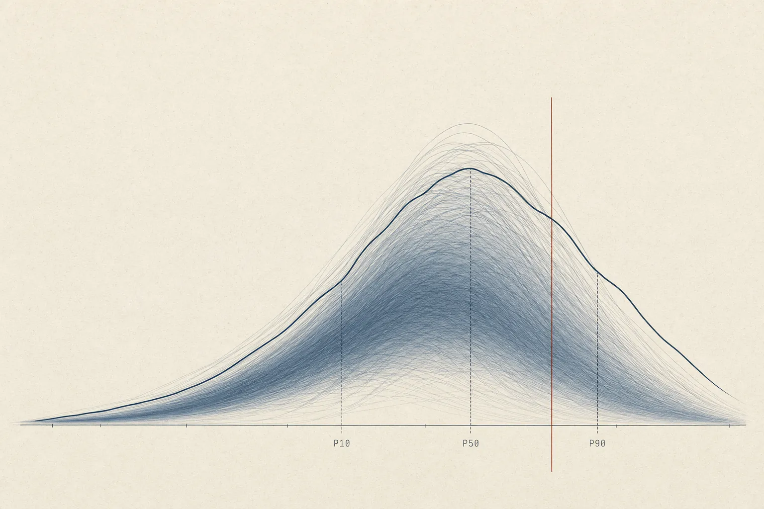
The headline
The chart below is the only one in this post that directly answers the question in the title. Every dot is a trial; the x-axis is Searcher implied IRR, computed against a $3M W-2 NPV counterfactual — i.e. the rate at which a ten-year search-fund cash stream beats the salary that same person would have earned otherwise. Zero is break-even with the outside job. Across 500,000 trials, the median is roughly –5%; the 90th percentile is +25%; the 10th percentile is the catastrophic –50% floor (a no-acquisition outcome with two years of search burn against an unchanged counterfactual). About 43% of trials clear zero. About 23% clear 10%. The shape of that mass, not the mean of it, is the question.
Searcher implied IRR vs. a $3M W-2
Distribution of Searcher implied IRR against a $3M Searcher equity value NPV counterfactual across 500,000 trials. P10 -50%, P50 -5%, P90 +25%. Roughly 43% of trials clear zero (beat the salary); ~23% clear 10%; ~12% clear 20%.
The center of mass sits below break-even, so the default case is not "you win" even when the right tail is real.
Pre-tax framing. Every dollar figure in this post is pre-tax. Stanford reports the asset class pre-tax, so the calibration is apples-to-apples — but actual take-home is roughly 25-37% smaller than the NPV figures here. Layer your own marginal rate on before reading the histogram against your personal hurdle.
How the company gets there
The histogram is the destination. The fans below are the road. Revenue, EBITDA, and the searcher's annual pre-tax cash flow over the full path — search years, operating years, exit. The shaded band on each is the P10–P90 spread; the dark line is the median trial. Read them in order: top-line first, then margin compounding into EBITDA, then how that flows to the searcher in cash and equity.
Revenue, acquisition to exit
P10 / P50 / P90 revenue bands across the operating period. Top-line spread is wide because customer count, churn, and ARPU all sample independently each trial; pair with the EBITDA fan below to separate top-line growth from margin evolution.
EBITDA, acquisition to exit
P10 / P50 / P90 bands of EBITDA across the operating period. The 80% band widens sharply by year five — variable cost, wage growth, and overhead compound; small differences in the operating model decide whether year-five EBITDA is twice the entry number or below it.
Searcher annual cash flow, end-to-end
P10 / P50 / P90 of the searcher's annual pre-tax cash flow across the full path. Years 1–2 are flat search salary, years 3+ are CEO base plus bonus, and the final year carries the equity-at-exit bolus — which is where most of the dollar value lives, and most of the variance.
Searcher pre-tax NPV at 9%
Distribution of searcher pre-tax NPV across all 500,000 trials. P10 $0.26M, P50 $1.46M, P90 $8.32M, mean $3.50M. The mean sits above the median because the right tail does most of the work — about 27% of trials clear the $3M counterfactual reference line.
The critical pattern is mean-median separation: the average outcome looks strong because a relatively small right tail carries a disproportionate share of value. If your utility cannot tolerate needing tail outcomes to beat your counterfactual, treat this as a pass even when expected value screens positive.
Drivers
This chart answers which inputs actually move the answer: flex each driver from its 10th to its 90th percentile while holding everything else fixed, and rank by the swing in median Investor IRR. Most drivers do almost nothing; a small handful do almost all the work.
Which drivers actually move Investor IRR
Each driver flexed from its 10th to 90th percentile, all others held at mean; bars sorted by the swing in median Investor IRR. New-customer rate dominates by a wide margin; entry multiple, debt percentage, and exit multiple cluster behind. Variable cost and hold years barely register.
The dominant pattern: commercial upside drivers create most of the distributional spread, while many operational levers mostly tighten around the middle. Pursue only if you can point to a concrete customer-acquisition edge before signing up for search risk; otherwise assume you will land near the center of the distribution, where the W-2 often wins.
The decision rule
Use this compact checklist (calibrated to the default $3M W-2 counterfactual):
- P50 Searcher implied IRR ≥ +5%. If median is below +5%, treat base-case economics as too thin.
- P(Searcher NPV > counterfactual NPV) ≥ 55%. If the beat-probability is near a coin flip, default to the outside option.
- Downside bucket share (no acquisition + loss buckets) ≤ 40%. If downside mass is above 40%, risk concentration is likely too high.
Uncertainty buffer: if any metric is within ±5 points of its threshold, treat the call as unresolved until the assumption set survives slower customer adds, higher leverage cost, and lower exit multiple.
Run it yourself
The canonical charts above are fixed at 500,000 trials so the article has one stable answer. The sandbox below runs a smaller 50,000-trial version in the browser so you can test how the decision changes when the entry multiple, leverage, hold period, discount rate, W-2 counterfactual, and volatility move.
Searcher implied IRR under your assumptions
Live-updating histogram of Searcher implied IRR for an in-browser run using the slider values. The vertical reference line marks break-even against the chosen counterfactual.
How the simulator is built
Five implementation choices matter for interpreting the static charts. The point is not to hand the reader a modeling tool; it is to make clear what the canonical output is doing under the hood.
- Engine. Tier-A LBO in Rust. Three vesting tranches (time / acquisition / performance with explicit IRR-hurdle step function), search capital 1.5× step-up, full senior debt amortization, seller note as subordinated tranche, idiosyncratic stress-event mechanic with persistent customer-count haircut.
- Operating model. 12-driver bottom-up SMB chassis (above). Customer cohort dynamics, ARPU evolution, cost build, capex and working-capital drag. EBITDA growth and margin are emergent.
- RNG.
Xoshiro256PlusPlus, seeded per-trial so order-of-execution doesn't affect results. Default seed is0xB06DA1DEC1DE; canonical JSON is byte-stable across builds. - Parallelism. The internal native build uses
rayon; the static 500k-trial dataset is generated offline and served as fixed chart data. - Calibration. Inverse-design — driver distributions are tuned so emergent (margin, growth, bucket) distributions match Stanford 2024 within the tolerance bands discussed above.
Model assumptions & limitations
- Pre-tax framing only. All simulator outputs are pre-tax; use your own tax stack before comparing model NPV/IRR to personal take-home hurdles.
- Calibration is in-band, not exact-fit. Treat outputs as calibrated ranges rather than point-precise forecasts.
- Single-regime chassis. Current calibration uses one generic SMB driver regime; sector-specific cyclicality, regulation, and technology risk are outside this release scope.
- Not industry-specific (yet). The current chassis parameterizes businesses generically.
- Counterfactual is fixed, not a distribution. The outside-option NPV is $3M in the canonical charts.
Use this as a decision aid, not a forecast.
Reference context the simulator does not see
Two context layers sit above the 12-driver chassis and bound what this simulator can claim. First, industry selection: the engine assumes you already filtered into a fundamentally desirable business profile before acquisition. Second, CEO cash compensation: the operating-year cash outputs should stay close to Stanford's published compensation curve as a realism guardrail.
What "buy a good business" actually means
The Stanford Primer's canonical desirable/undesirable matrix is the pre-filter for this model. The simulator assumes you acquired a business in the desirable column, with the practical sweet spot around $1.5–$5M EBITDA, >15% margins, limited concentration, and durable recurring revenue.
CEO base + bonus through hold period
Stanford's published CEO cash-compensation curve is used as an external realism check. The operating-year cash line in Exhibit 4 should stay directionally consistent with this tenure profile; if it drifts too far, the searcher cash-flow fan is likely mis-specified.
| Years since acquisition | Base mean | Base median | Bonus mean | Bonus median | Total mean | Total median |
|---|---|---|---|---|---|---|
| ≤ 1 | $187k | $190k | $29k | $25k | $217k | $200k |
| 1–2 | $212k | $210k | $49k | $55k | $263k | $262k |
| 2–3 | $217k | $215k | $44k | $50k | $261k | $265k |
| 3–4 | $220k | $225k | $59k | $67k | $289k | $292k |
| 4–5 | $209k | $205k | $40k | $29k | $249k | $226k |
| > 5 | $256k | $229k | $75k | $45k | $336k | $260k |
What the full picture actually says
The headline number from 500,000 trials is uncomfortable: the median searcher comes out roughly 5% per year worse than if they had stayed in a high-paying job. Not 5% worse in absolute dollars — 5% per year, compounding, over the full duration of the search and hold period. That is a bad number. About 43% of trials beat the alternative of keeping the corporate career — taking the salary, skipping the search risk, and compounding steadily. The mean looks better than the median because a relatively small right tail carries most of the aggregate value — and that is precisely the pattern that warrants careful reading.
None of this means search funds are a bad idea. It means they are a concentrated bet that requires a concrete reason to believe you will be one of the few who actually wins big — not a generic instrument that works for any talented person who is tired of their current job.
Here is the checklist that actually matters.
Go if
You can absorb two-plus years of search salary — roughly $100k–$140k — while your W-2 peers compound. The opportunity cost is real and starts immediately; the equity is back-loaded and uncertain.
You have a sourcing or customer-acquisition edge you can articulate before you start. The tornado chart (Exhibit 5) makes this unambiguous: new-customer rate is the single dominant driver of outcome dispersion. Industry skill, proprietary deal flow, a credible operator network — these things move the distribution. Analytical ability alone does not.
You can point to a specific type of business in a specific industry and explain, from first-hand experience, why you can run it. The failure modes in Section 1 are almost all operator-fit failures: the searcher bought a business that needed a frontline executor, then discovered too late that they were an analyst. That mismatch does not surprise anyone who examines it honestly in advance.
Your best W-2 alternative genuinely does not appeal to you for the next decade. This is not "I'm burned out right now," which is a present-tense state that usually resolves, but "I actually do not want to be an employee of a large institution for the next ten years." The analysis draws a straight line between that preference and the search fund upside; the line is long.
Pass if
The main draw is financial upside. The right tail is real — and in dollar terms, it is significant. The 5–10× bucket (about 11% of acquisitions) typically means the searcher walks away with $5M–$12M pre-tax. The >10× bucket (about 5% of acquisitions) means $14M–$25M or more. Those outcomes exist and are not flukes. But 12% of all concluded search funds land there, and they are not randomly distributed across searchers. If you are optimizing for wealth creation and the search fund is primarily an investment vehicle in your mental model, you are probably better served by a direct path into buy-side investing or private equity where the same skills earn competitive returns without the operating-company risk.
You are doing this to escape something rather than to build something. Burnout is a real signal that deserves a real response. It is not, by itself, a reason to take on two years of search risk, significant leverage, a decade of CEO accountability for a small company in a boring industry, and a distribution with a median below break-even.
You cannot name a specific business type, in a specific industry, where you have a genuine operating edge. "I'm good at analysis" describes most people who look at search funds. The distribution is not impressed.
One last note.
Everything in this post is pre-tax. Stanford reports the asset class pre-tax; the calibration is apples-to-apples. Your actual take-home is roughly 25–37% smaller than the NPV figures here. Run your own numbers through your own tax stack and your own W-2 counterfactual before treating any of this as a decision — that is why the sandbox in Section 5 exists.
QSBS. Qualifying U.S. C-corp deals can exempt the greater of $15M or 10× basis per shareholder from federal capital gains, which materially compresses the equity-at-exit haircut on the NPV figures above. Worth structuring for early. Source: Stanford Search Fund Primer (2026), p. 23.
The simulator is calibrated to Stanford's published cohort data, but the fit is close, not exact — see Exhibit 1 for the bucket-level diagnostics. Treat outputs as directional ranges, not point forecasts. Use the decision rule in Section 4 as a framework, not a formula.
Notes and sources
- Pre-tax framing. Every cash figure in this post and in the underlying simulator is pre-tax. Stanford's 2024 study reports the asset class pre-tax, so the calibration is apples-to-apples — but actual take-home is roughly 25–37% smaller than the NPV figures here. A rough conversion: federal + state ordinary on cash comp (~35–40% effective at a high-income bracket), federal LTCG + state on the equity-at-exit bolus (~20–25%), so the blended haircut on the searcher NPV runs ~25–35% depending on the ratio of cash-to-equity in the path.
- Calibration tolerance. The simulator's emergent bucket frequencies match Stanford's published frequencies to within ±3.6 percentage points on every bucket; total absolute deviation is ≈14pp. Tightening past this requires either a multi-regime mixture model or industry-specific operating chasses; both are follow-up extensions beyond this baseline model. Visible in Exhibit 1.
- Counterfactual NPV default. The $3M default is the fixed 10-year W-2 NPV benchmark used throughout this post, pre-tax, discounted at 9%. The model does not draw a counterfactual distribution; that is a different, harder modeling exercise.
- Catch-up clauses (not modeled). The 2026 Primer documents a catch-up mechanism where, after performance benchmarks are met, the searcher recovers the coupon paid on investor preferred equity — the worked example shows an effective 78/22 split (driven by the 8% coupon) "canceled out" back to the agreed 70/30. Our simulator does not model this; including it would shift the right tail of the searcher NPV histogram by an estimated 2–5pp of searcher IRR in good outcomes. Source: Stanford Search Fund Primer (2026), pp. 18–19.
- Super carry / equity kicker (not modeled). The 2026 Primer names an explicit "home run tranche" of bonus equity awarded at 35–40% IRR or 5–10× MOIC. Our model treats equity-at-exit as a single waterfall and does not break out the kicker; the omission understates searcher upside in the >10× bucket where the right tail actually lives. Source: Stanford Search Fund Primer (2026), p. 22.
- Model taxonomy. The three-way split in Exhibit 0 — Traditional / Self-Funded / Sponsored — is drawn from Models of Entrepreneurial Acquisition (Stanford E-365, 2011, pp. 4–10), with the Traditional column cross-referenced against the Stanford Search Fund Primer (2021, pp. 7–18). Anchor cases (Brown Robin / OnRamp Access; Sanabria / Impress Northwestern; Callahan / YLighting) are the case studies in the same MEA document.
- Cohort drift. Exhibit 1c reports per-2-year cohort medians from Stanford GSB 2024, Exhibit 5 (p. 20). The "All" column is the pooled median across all acquisition years (n=324 closed deals reporting purchase price, per Exhibit 6, p. 20). The drift in PP/EBITDA from 5.2× (06–07) to 7.0× (22–23) is the multi-cohort version of the median sanity check in Exhibit 1b.
- Primary source roll-up. Stanford GSB 2024 supplies the outcome tree, deal-level medians, CEO compensation curve, and cohort drift. Stanford GSB 2022 back-fills the 2009 row in the outlier-dependency table. Stanford Search Fund Primer (2021) supports the search funnel and industry rubric; Stanford E-365 supports the model taxonomy.
- Additional source notes. IESE Business School 2024 is used only for LOI failure modes in Exhibit 1g, not for an international return comparison. Columbia Business School S3 supports the time-allocation profiles. Overton Collective supports the direct-mail sourcing datapoint. Yale search-fund materials were used as methodology cross-checks on the LBO chassis and post-close CEO checklist.
- Stanford Search Fund Primer (2026 edition). Supersedes the 2021 edition cited above. Page references in this post correspond to the 2021 edition that was current at the time of writing.
-
Reproducibility. The canonical 500k-trial JSON is
served at
/data/search-fund-mc.json. The page renders that fixed dataset and does not expose a reader-run simulation.